ML Powered Autonomous Forecasting with SAP IBP for Demand

Hello all,

Sales Teams or Demand Planners are often not able to look beyond the top N high ASP / high Volume SKUs and also the demand planning cycles end up being focused on mostly just the upcoming quarter. Machine Learning offers the promise of accurate forecasts at scale and across the full forecast horizon, but cannot see round the corners as well as humans can in these non-linear and turbulent times. This presents an ML adoption conundrum, when it comes to autonomous forecasting. Hybrid approaches that blend human and machine intelligence in a pick-the-best-athlete mindset SKU by SKU quarter by quarter produce better outcomes than either a fully human or fully machine automated processes. Best part is the SKUs/Quarters where Machine drives the forecast in a fully autonomous manner gets dynamically dialed up / down in direct proportion to machine performance in delivering robust demand signals, thus minimizing risk, while letting humans remain in control throughout.

This blog presents one such hybrid modeling approach in SAP Integrated Business Planning IBP solution to enable this best-of-breed autonomous forecasting capability. We show how a composite forecast signal can be generated across the best ML signals and human judgment based forecasts from Account Teams / Demand Planners. Machine Intelligence can range from Gradient Boosting within SAP IBP and other more advanced models such as Neural Networks (Deep Learning or the true AI) outside IBP.  The design intent is to generate the most accurate composite signal by SKU by quarter across machine and human intelligence, while automating the composite signal generation based on business defined guardrails. It also contains best practices for conducting Machine Learning Pilots / POCs to quantify the forecast accuracy improvement potential across full data sets.

GitaCloud team recently conducted one such full-scope Machine Learning pilot for a High-Tech customer. In this case, the ML Pilot scope included both Demand Forecasting and Demand Sensing within SAP IBP as well as custom ML models outside SAP IBP for all the products for a given Business Unit of the High-Tech Customer. GitaCloud has industry specific process best practices models: see one such example below for Planning Processes in High-Tech, powered by Machine Learning capabilities. You may have to zoom the picture to understand how ML can enable next-gen capabilities such as Demand Shaping & Optimization on top of the typical Demand Sensing / Forecasting use cases.

Let’s discuss some of the details of this ML Pilot. Customer shared their sales forecast and consensus demand plan snapshots across last 36 historical monthly lags. Quick refresher on the concept of lag in IBP: forecast generated in July cycle for July is lag 0, for August is lag 1, for September is lag 2, and so on. Customer also shared historical bookings, historical constrained supply plan snapshots, channel inventory, and sales out data. We set-up the Gradient Boosting for Decision Trees GBDT Model in IBP Demand Forecasting along with ARIMA, Auto Exponential Smoothing, and Croston TSB in a MAPE based pick-best model selection approach. We also deployed custom ML models using Python outside IBP and loaded the corresponding custom ML forecast into IBP for composite forecast generation (pick-best across IBP and Custom ML models along with user forecasts).

Lag snapshots and other data sets need to be extracted from customer systems into flat files. A best practice here is to provide field by field explanations, sample data, and template files to Customer’s IT Team and explain why you need the data the way you are requesting it. In our case, we had to create full Excel mocks across multiple monthly cycles to explain how lag snapshots work and how ML models were going to use these datasets. In our experience, this minimizes the risk of incomplete or incorrectly extracted data, as it can be painful to discover foundational issues with data extraction half way into the pilot engagement. Plan on significant data validation / clean-up effort and 2-3 iterations of extraction before you get the minimally acceptable data quality to be able to produce robust ML signals.

We received historical bookings data at sales order line item level detail and loaded this data using flat file at a DAYCUSTOMER planning level (Day – Sales Order – Line Item – Schedule Line as keys), which we then aggregated to MTHPRODLOCCUST Month-Product-Location-Customer level. We defaulted location and customer to a single value across the board as the focus was to forecast the Demand for Products on a global basis. We also loaded sales forecast and consensus demand plan lag snapshots across 36 lags. We noticed a high number of duplicate records in the user forecast lag snapshots as the monthly planning cycles sometimes took place twice within the same fiscal month definition. This led to IBP rejecting data and ending up with holes in data in back to back months. This increased the forecastability challenge as the historical bookings data was already quite intermittent.

We calculated error as Absolute Percentage Error (APE) at Product level, then calculated Mean Absolute Scaled Error (MASE) across Products with bookings quantity acting as the weight in the weighted averaging of error.

We modeled fiscal time periods for this experiment with a fiscal calendar running from February to January. We were provided historical bookings data till February 2022 (which maps to fiscal month 1 of fiscal year 2023). We decided to run historical forecasting cycles monthly starting April 2021 (which is fiscal month 3 of fiscal year 2022). Intent was to capture lag 1 forecasts across monthly cycles and then compare error in quarterly buckets. See picture below to understand the forecasting methodology better.

Note how monthly forecasts for lag 1 were put together to generate the quarterly forecast: April cycle forecast for May, May cycle forecast for June, July cycle forecast for July make up the fiscal Q2 (May-July). We developed fiscal Q3 (August – October 2021) and fiscal Q4 (November 2021 – January 2022) forecasts the same way.

We developed a lag 1 Naïve Forecast using Single Exponential Smoothing model. We then calculated Forecast Value Add FVA by subtracting IBP Forecast MASE Error from Naïve Forecast MASE Error. We did the same FVA calculation for custom ML Forecast, for sales forecast, and for consensus demand plan lag 1 error. This helped us identify a lag specific FVA Winner across the competing forecasts. We developed a composite forecast based on defaulting the corresponding forecast based on the FVA Winner for a given lag. For example, if lag 1 Sales Forecast was the highest FVA historically (average FVA for the last 6 months) for a given SKU, then we will default the Sales Forecast into the Composite Forecast. We may choose to default IBP Forecast into the composite forecast for lag 4, if IBP FVA historically for lag 4 was the highest.

This helps planners to leave alone SKUs and/or a subset of forecast horizon (represented by specific lag values, e.g., lag 4-12) to default based on IBP ML forecast or the custom ML forecast. This helps move the forecasting process towards autonomous forecasting as SKUs and time frames forecasted more accurately by machines are left alone, while Business Users keep the focus on high ASP / high revenue SKUs. The system is self-learning as the FVA Winners and all the competing forecast snapshots can be fed into the Machine Learning ML Model to learn which SKUs are doing well by which stakeholder group and dial forecast automation up or down autonomously. For example, an SKU which was earlier being defaulted from custom ML forecast may switch back to user forecast, if it exceeds a threshold for forecast error or gets into the top 20% of the product portfolio from a revenue contribution perspective.

We recommend to drill down into examples of SKU level extreme error and visualize all relevant datasets in an Analytics view to understand root causes of the high error. This can range from unforecastable data series with significant intermittency or a data integrity issue with forecast snapshots missing data due to duplicate records rejected by IBP. We found it useful to model multiple instances of Gradient Boosting model with different combinations of parameters such as # of trees, tree depth, etc. within the same forecast model overall. You will want to store all model specific forecasts in dedicated key figures to understand which model is working well for which SKU as a clue into further fine-tuning of model parameters. Also play with different values of preprocessing methods and parameters, as the outlier correction had a significant bearing on forecast error in our specific data set. We also recommend playing with the Gradient Boosting Global parameter Disable_Hybrid_GBDT to X to see if this helps.

We recommend running Forecast Automation Job in IBP and checking off the box on ‘Consider Time-Series Properties’ in IBP Forecast Model definition.

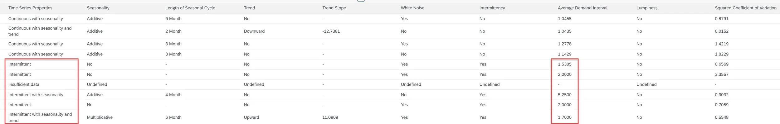
See a sample of results from Forecast Automation run in IBP: IBP can identify intermittent SKUs with trend / seasonality patterns and report key parameters such as Average Demand Interval to aid Demand Planners in understanding Demand Pattern mix across a large SKU portfolio.

Given the need to run 10 monthly cycles historically and take snapshots across multiple experiments, we created an application template with all the jobs in a well structured sequence. You can set forecast jobs to run on a historical date by selecting specific dates for forecast steps in the template as shown below. This organization of forecast steps in a template helps with experimentation speed and rigor in configuration management. We had 152 steps in our template and found the ability to copy template into additional versions with a forecasting model change in a subset of steps as a very efficient way to deal with configuration management during the high number of experiments we ran.

We recommend maintaining an application template change log to note exactly what’s different in each application template and how it’s evolved and tie all application jobs back to these templates. We experienced model drift at several points during the experimentation and the change log helped to get back to precise configuration choices that had produced lower error in our earlier experiments.

Hope this gives you a good sense of how to enable Autonomous Forecasting powered by SAP IBP for Demand. GitaCloud is happy to help customers across High-Tech and other industries validate hard business value from Machine Learning / Deep Learning applications in Demand Forecasting domain.

A typical full scope ML Pilot takes GitaCloud team just 4-6 weeks to deliver. Customer needs to decide what they wish to forecast (bookings, shipments, revenue, etc.) and in which time frame (tactical, operational, etc.). We need to understand the current Forecast Error Metric and finalize the Error Metric and Calculation Method to use for running the Pilot (which level, what lag, what time granularity, etc.).  Customer IT teams need to share relevant data for the last 3-4 years in flat files shared in a secured shared folder. This can include Product Master (Hierarchy Attributes), Historical Bookings / Shipments / Revenue, Historical Forecast Lag Snapshots, Historical / Current Pipeline, Historical / Planned ASPs, Historical Snapshots of Constrained Supply Plans, Sell-Out History, Channel Inventory, etc. All sensitive data can be anonymized, no confidential identifying details such as product description need to be shared. Product hierarchy attributes and Geo values can also be anonymized, as needed. Customer should keep aside the last quarter of historical values to assess quality of ML forecast solution post Model training. It’s critical to define quantitative success criteria upfront, to ensure they can be validated with help from forecastability analytics (which is a topic for another blog).

You can always reach out directly to me at ashutosh@gitacloud.com, if you would like to get a similar bottoms-up quantification of the forecast value add from Machine Learning within / outside SAP IBP, or if you have any questions regarding the  solution approach presented here.

As always, good luck with your endeavors in delivering exceptional customer success and value through your SAP IBP or S/4HANA powered supply chain transformation engagements.