Configurable Products Planning: SAP IBP Enhancement for Make To Order MTO Industries

Hello all, this blog is focused on how to plan configurable products in SAP IBP. This is an enhancement delivered by GitaCloud team to augment S/4 Add-On for SAP IBP interface to support both Time Series Planning TS) and Order Based Planning OBP in SAP IBP. Read content below to understand the business requirement, SAP IBP functionality gap, solution approach, and business value, when it comes to planning configurable products in SAP IBP.

Introduction:

• Make To Order MTO industries often deploy Variant Configuration within SAP S/4HANA to support sales order specific product configurations.

• This helps to avoid the product proliferation issue in S/4. However, S/4HANA does not integrate currently with SAP IBP for sales orders with variant configuration (material type: KMAT).

• As you may know, S/4 Add-On for IBP enables both master data (products, customers, suppliers, BOMs/Routings, etc.) as well as transaction data (sales orders, stock, production orders, purchase orders, etc.) to be integrated via batch jobs into SAP IBP.

• S/4 Add-On for IBP can be leveraged to support both Time Series Planning using SAP IBP S&OP application as well as Order Based Planning using SAP IBP Response & Supply application.

• SAP IBP Response and Supply Application supports an Order Based Data Model tightly integrated with SAP S/4HANA. This enables Order Based Planning OBP capability in SAP IBP: which helps in combining the MRP and ATP processes with a single planning run in IBP: to support both Sales Order Confirmations and Planned Order / Purchase Requisition generation for execution in S/4HANA.

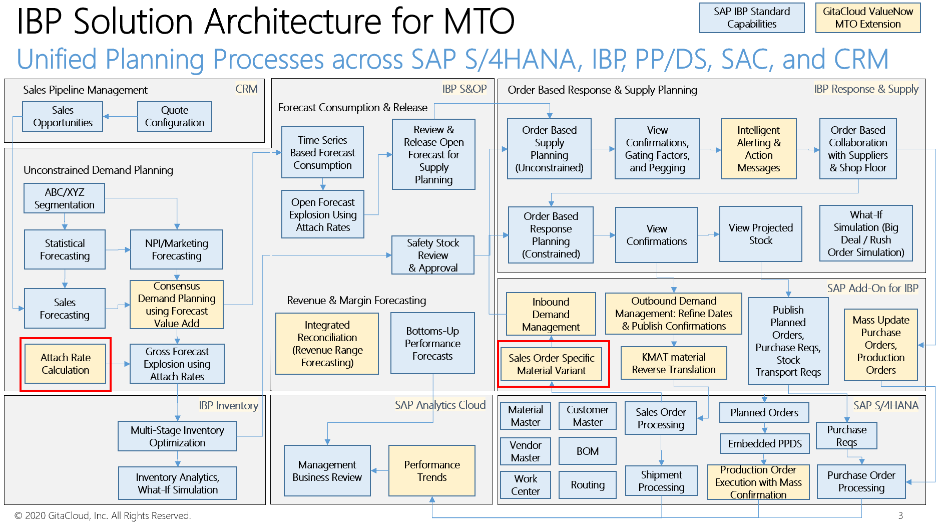
• This enhancement is built on top of the standard S/4 Add-On for IBP. With this Configurable Product Planning enhancement developed by GitaCloud team, planners can support TSP processes like Statistical Forecasting, Consensus Demand Planning, Forecast Consumption in IBP S&OP for configurable products. Planners can also support Sales Order Confirmation and Order Based Supply Planning for configurable products to replace MRP and ATP processes in S/4.

• See end to end Solution Architecture view for Make To Order MTO below, before we deep-dive into the Integrated Business Planning for MTO solution.

Business Requirement:

• Make To Order industries have a high degree of product function/feature variability associated with every sales order. Creating each of these product requirement flavors as a distinct material in S/4 is not desirable, as the odds for a re-use of this product definition are low, and it leads to unnecessary product proliferation in terms of master data volumes in S/4.

• Planners are challenged to execute typical Time Series Planning (S&OP) processes for configurable products given the shifting Bill of Material for every incoming sales order. Planners usually manage a Forecasting/Planning oriented BOM in S/4, which lists all the possible options on the BOM, then manage attach rates as Qty Per to forecast BOM components somewhat accurately.

• Please note that Make To Order MTO does not mean that planners can start planning from scratch when the sales order comes in. The cumulative lead time for procuring the sales order specific BOM for all the procured components and to go through the multiple levels of assembly in the production shop floor often exceed the order lead time (time the customer is willing to wait from the order placement to order delivery). This means Planners have to balance the inventory risk with the customer service risk: buy too much and finance is unhappy; buy too little and sales is unhappy.

SAP IBP Capability Gap:

• SAP offers Variant Configuration VC capability or recently, Advanced Variant Configuration AVC capability to manage sales order level product definition.

• SAP does not currently support VC sales orders to be integrated into IBP through the S/4 Add-On for IBP.

• Given the attach rates can vary greatly over time, it is quite a challenge for planners to maintain the Forecasting/Planning BOMs to drive material requirements in a balanced manner. Attach rates need to be calculated based on recent shipment history and be made available to Planners as Decision Support.

GitaCloud Solution Enhancement: Configurable Products Planning

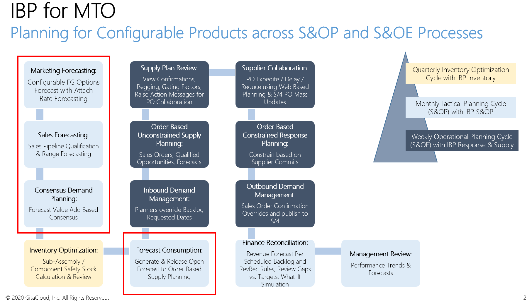
• See overall IBP Process Flow view below to understand how quarterly-monthly-weekly planning processes integrate to support Integrated Business Planning for Configurable Materials in Make To Order industries. We will focus on the Time Series Planning Processes in this blog.

• Shipment History: Let’s use a detailed example to explain the nuances of the solution. Let’s take a configurable material in S/4 called KMAT1 (material type: KMAT stands for configured materials).

• Each Sales Order (SO) shipped has a main line item, where the KMAT1 material is recorded.

• Let’s go with a simple Variant Configuration model where customers can select option numbers ranging from 1 to 10. Each option selected drives the corresponding lower level sub-assembly in the sales order specific Bill of Material BOM.

• The sales order configuration is shown with lower level line items in the SO (and carry the main line item of KMAT1 in the High-Level Item # field as per snapshot below.

• See snapshot below to see shipment history data for last 12 months. For example, SO# 501 has a main line item # 10. Ship-to Customer 50001 has asked for Option # 1, 3, and 4 in this case. This drives KMAT1-SUBASSY1, KMAT1-SUBASSY3, and KMAT1-SUBASSY4 as lower level line items (item # 20, 30, and 40), all of which have High Level Item # field as 10 to point to the main line item for KMAT1.

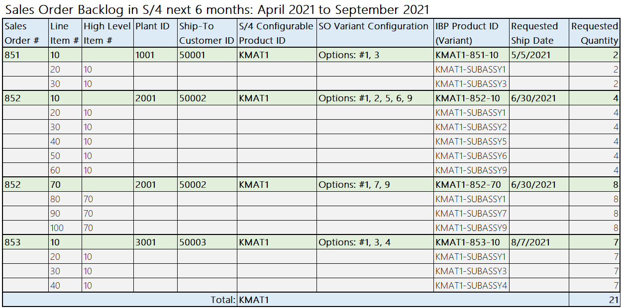
• We also load Sales Order Backlog (open orders) the same way into IBP per snapshot below.

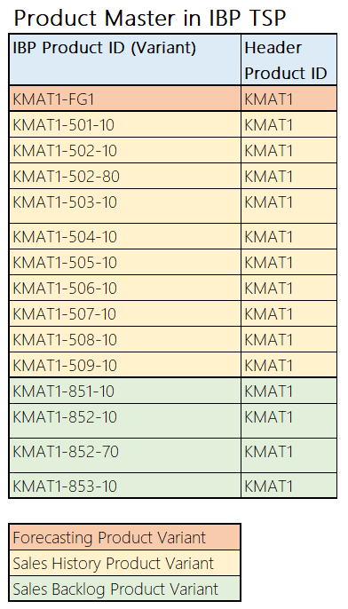
• Product Master Modeling Approach: We load Shipment History at a Sales Order Line Item level in IBP Time Series Planning (IBP S&OP or IBP Demand) in a custom Master Data Type MDT. Each instance of a unique configuration of KMAT1 is modeled into IBP TSP with a unique material variant by concatenating the SO # and Line Item # to the configurable product #. For example, we create an IBP Product ID called KMAT1-501-10 to store the unique configuration of SO # 501 Line Item # 10 in its BOM. IBP Product Master MDT has an attribute called Header Product, where all such SO specific unique product variants get the same configurable product value, i.e., KMAT1.

• We also create a Forecasting/Planning relevant Product ID as a regular Finished Good material in S/4 (material type: FERT): KMAT1-FG1. Planners use this product to forecast demand for KMAT1 configurable product.

• See IBP TSP Product Master MDT below to understand all the products created across Shipment History, Sales Order Backlog, and the Forecasting/Planning relevant Product.

• Attach Rate Calculation: We calculate the % of the time a specific option was ordered in the last 12 months, when a given configurable product was ordered. We refer to this as Attach Rate. This is calculated monthly on a rolling last 12 months basis.

• For example, KMAT1 total quantity shipped in the last 12 months (April 2020 to March 2021) is 65 units in the Shipment History dataset above. See table below to understand the computed attach rates by each VC Option (which drives a specific sub-assembly in our example). As Option # 1 (default base unit) is always ordered, its attach rate is 100%. As Option # 2 was ordered in a total quantity of 17 units, its attach rate is 17 divided by 65, which comes to 26%.

• Bill of Material BOM Modeling Approach: Planners maintain a Forecasting/Planning Product specific BOM in S/4 manually based on the calculated attach rates.

• Planners need to retain manual control of the BOM definition and define attach rate in the Qty Per field of the BOM freely, to support the following scenarios:

  • Attach Rate Override: Marketing Team or Planners may be aware of planned pricing or option bundling strategies, which may result in future attach rates being different from the past.

  • New Options: New options may be introduced and need to be planned, but are not present in the shipment history.

  • Obsolete Options: Options that sold in the past may also be discontinued, in which case the corresponding option needs to be deleted from the component list in the Forecasting/Planning BOM.

• See the table below for the Forecasting/Planning Product’s BOM with Attach Rates. This BOM is created manually and flows into IBP IBP Order Based Planning OBP through the standard S/4 Add-On for IBP: no solution enhancement required.

• Note the Option # 10 (which drives the KMAT1-SUBASSY10 part was not sold at all in the last 12 months. Attach Rate was calculated as 0% for this part. However, Marketing Team has decided to put a pricing promotion for this option and expect a 10% attach rate going forward. This is reflected as Qty Per being 0.100 for 1 unit of the output product KMAT1-FG1.

• Also note that Marketing Team has also decided to launch a brand new option #11, which will drive the part KMAT1-SUBASSY11 with a planned attach rate of 5%. This is reflected in the BOM with Qty Per being 0.050 for the KMAT1-SUBASSY11 part.

• Sales Order BOMs for past shipments or open sales backlog are modeled based on the specific configuration: Qty Per is always 1 in this case and Attach Rate concept does not apply.

• See Sales Order specific configurations mapped as SO specific BOMs for the Shipment History in the S/4 Add-On for IBP. This is a solution enhancement developed by GitaCloud.

• See the table below for all the BOMs loaded into IBP Order Based Planning OBP: to support the Open Sales Order Backlog as well as Forecast for the Forecasting/Planning Product.

• Let’s focus on the Time Series Planning TSP business processes with this Master Data Modeling approach in IBP.

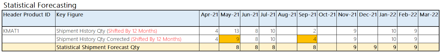
• Statistical Forecasting: Shipment History can be aggregated across all SO Line Items at Header Product level KMAT1. We shift the Shipment History by 12 months to make it easy for Demand Planners to see all Shipment History and Open Sales Order data in the same future horizon: from April 2021 to March 2022.

• Outlier Correction algorithms can be applied to correct the Shipment History, which is then also shifted by 12 months.

• Statistical Forecast can now be generated using SAP IBP S&OP (Basic Statistical Forecasting: Exponential Smoothing) or SAP IBP Demand (Advanced Statistical Forecasting: with forecasting algorithms such as ARIMA, Croston’s, Causal Forecasting, Gradient Boosting, Automated Exponential Smoothing, etc.).

• See snapshot below for Statistical Forecasting view in Excel Add-In for IBP. Note that Shipment History was corrected from 13 to 9 in May-20 (reflected in May-21 with the 12 month shift) and from 2 to 4 in Sep-20 (reflected in Sep-21 with the 12 month shift). Best Fit Statistical Forecast is highlighted below.

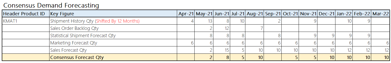
• Consensus Demand Planning: Let’s take a classic consensus demand planning process across Sales, Marketing, and Demand Planning Team. Marketing Team has a flatlined forecast of 6 units each month. This is based on a quarterly Marketing Plan of 18 units each quarter, which has been spread equally to 6 units every month. Looking at the erratic Shipment History pattern in this COVID-19 pandemic time, it is clear that Marketing Forecast is more geared towards annual revenue planning process, and does not help the Demand Planning team much in this case. Sales Forecast on the other hand is extremely aggressive with double-digit numbers in all future months despite having no sales orders due to ship in the current month of April 2021. Sales Forecast seems to be geared towards meeting Sales Quota, which are set by design to be 2x of expected revenue. Demand Planning Team can clearly see the risk with adopting this optimistic forecast. Demand Planning Team also looks into the CRM system for opportunity pipeline and notice an opportunity in August 2021 with a high probability to close (80%). Demand Planner decides to adopt this opportunity into the Consensus Forecast (10 units in August 2021, which are not reflected in the statistical forecast). However, Demand Planner reduces the forecast in July 2021 and in November 2021 to compensate for this.

• See below the view shared by Demand Planner in the Consensus Demand Review Meeting.

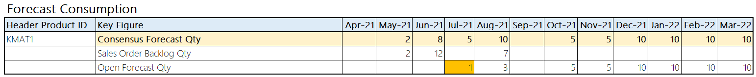
• Forecast Consumption: SAP IBP Response & Supply application is used to drive Order based Planning (OBP). We have turned off Forecast Consumption process in OBP, and consume the (gross) Consensus Forecast Quantity with Open Sales Order Backlog in the TSP side. Forecast Consumption is defined at the Header Product level: KMAT1. This enables an aggregated view of sales orders across all unique product variants.

• Note Sales Order Backlog is 12 in June 2021, which is higher than Consensus Forecast in the month of June 2021, which is 8. Forecast Consumption Mode in this case allows forecast to be consumed forward, hence 4 out of the 5 units forecasted in July 2021 are consumed. This results in the Open (Net) Forecast Quantity being just 1 unit in July 2021.

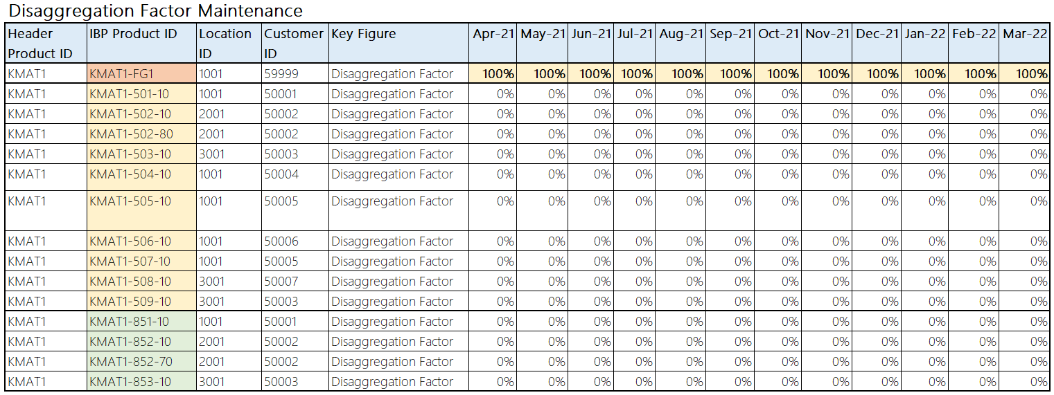
• Forecast Release: The entire TSP process from Statistical Forecasting to Consensus Demand Planning to Forecast Consumption has run at Header Product level till now. However, we need to release Forecast at Product ID level to OBP side (IBP Response and Supply application). We use the concept of Disaggregation Factors to allocate the entire Header Product KMAT1 level Open Forecast Quantity to the Forecasting/Planning Product KMAT1-FG1. Open Forecast Quantity Key Figure is set to disaggregate using this ‘Disaggregation Factor’ key figure. The disaggregation factor key figure is automatically populated from the CPI interface: 100% allocation to the Forecasting/Planning Product and 0% allocation to all unique Product Variants based on SO line items.

• See snapshot below to view the Disaggregation Factor key figure values populated by the CPI interface for the next rolling 12 months of forecast horizon.

• Open Forecast Quantity Key Figure is disaggregated from Header Product level to Product level automatically. The entire forecast is defaulted to the main location 1001 and to a default customer ID of 59999. This enables planners to consolidate procurement for all the forecast orders in the main plant: 1001.

• See snapshot below:

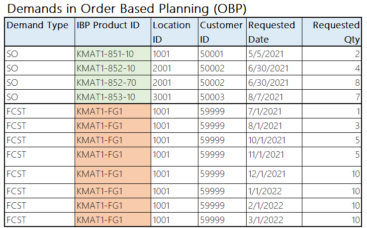
• Open Forecast Quantity Key Figure is exported using CPI and uploaded directly in S/4 Add-On for IBP tables, such as Order_Ext using a full refresh (remove old Forecast, load new Forecast). This enables Forecasts to be loaded technically as Sales Orders of type Forecast into OBP. This enables the capability of SO line item # granularity views in IBP Excel Add-In, which is not possible, if the Open Forecast is released directly from TSP to OBP as a Key Figure. See snapshot below to get a final view of all the independent demands in IBP OBP.

Business Value:

• This approach enables planners to precisely plan forecast with a planning BOM (using dynamic attach rates) and sales orders with sales order specific BOMs. This ensures all sub-assembly parts and lower level parts are manufactured or procured in the right amounts at the right time. This ensures an optimal balance between customer service and working capital / inventory optimization goals.

• These unique product variants are hidden from the user views in TSP Demand Planning processes, given the entire process runs at Header Product level. This aids usability for Business Teams, while retaining the ability to drill down to individual Sales Order Configurations in order to drive revenue planning and margin forecasting processes in a highly precise manner.

Conclusion: 

• Hope this gives you a good sense of the solution enhancement and value. It addresses a key interface / modeling gap from Configurable Products Planning Process perspective.

• GitaCloud has implemented a holistic approach to planning configurable products that works across the Time Series and Order Based Planning processes. GitaCloud has packaged this set of holistic solution enhancements as a branded offering: ValueNow for MTO.

• Reach out at connect@gitacloud.com, if you have similar unmet business process requirements with your current SAP IBP implementation or you would like to understand the solution better.